From the carbon cycle to forest disturbance scenarios: explore how organic inputs, climate and management shape soil carbon over time.
Start with the foundations
These guides introduce soil organic carbon (SOC) and take you through the steps needed to run RothC. Begin with the introduction, follow the practical guide, then apply the workflow in the workshop exercises.
Introduction to Soil Carbon & Environmental Modeling
This introductory guide explains the fundamental science behind Carbon, Soil Organic Carbon (SOC), and Carbon Dioxide (CO2), as well as why computer models like RothC are vital for predicting soil health and climate impacts.
1. Why Carbon, SOC, and CO2 Matter for the Environment
Carbon is the fundamental building block of life on Earth, constantly cycling between the atmosphere, oceans, vegetation, and soils in what is known as the global carbon cycle.
- Carbon Dioxide (CO2) and Climate: CO2 is a primary greenhouse gas in Earth's atmosphere. While natural levels keep the planet warm enough to support life, excess atmospheric CO2 from human activities (fossil fuel combustion and land-use change) traps heat, driving global climate change.
- Soil Organic Carbon (SOC): SOC represents the carbon stored within soil organic matter—the decayed remains of plants, roots, microbes, and animal material. Soil is Earth's largest terrestrial carbon reservoir, storing more carbon than the atmosphere and all living vegetation combined.
- Soil Health and Ecosystem Services: Beyond storing carbon, high levels of SOC improve soil structure, enhance water retention during droughts, boost nutrient availability for crops, reduce soil erosion, and support diverse soil microorganisms essential for agriculture.
THE WIN-WIN OF CARBON SEQUESTRATION
Soil Carbon Sequestration is the process where atmospheric CO2 is absorbed by plants through photosynthesis and stored long-term in the soil as organic carbon. Transferring carbon from the atmosphere into agricultural soils simultaneously tackles climate change and rejuvenates farmland productivity.
2. Why Do We Want to Model SOC?
Measuring SOC through physical soil sampling requires field visits, lab analyses, and chemical tests. While indispensable, field testing alone has critical limitations that make computer modeling essential:
- SOC Changes Slowly: Changes in soil carbon occur over years or decades. Measuring these shifts in a laboratory year-to-year is difficult due to background noise and natural soil variability.
- Predicting the Future: Field measurements can tell us current soil carbon stock, but they cannot predict future outcomes. Models allow scientists and land managers to test "what-if" scenarios over 30, 50, or 100 years.
- Evaluating Management Practices: Modeling makes it possible to evaluate agricultural practices (such as cover cropping, reduced tillage, compost additions, or agroforestry) and identify which strategies maximize carbon sequestration before investing resources in the field.
- Regional and Global Policy: Models allow governments and organizations to estimate carbon sequestration potential across whole regions, countries, or continents to support carbon markets and agricultural policies.
3. What Are SOC Models and What Is RothC?
An SOC Model is a mathematical representation of chemical and biological soil processes. By providing inputs—such as historical weather, land cover, soil physical traits (e.g., clay content), and organic inputs—the model simulates how microbial decomposition breaks down organic matter and releases or retains carbon over time.
The Rothamsted Carbon Model (RothC)
RothC (short for the Rothamsted Carbon Model) is one of the world's most established, tested, and widely used soil organic carbon models. Originally developed at the Rothamsted Research institute in the United Kingdom, it simulates the turnover of organic carbon in non-waterlogged topsoils.
The 5 Carbon Pools in RothC
Unlike simple models that view soil carbon as one uniform block, RothC splits total SOC into five distinct pools based on how resistant they are to microbial decomposition:
| Pool Code | Pool Name | Decomposition Rate ($k$, $\text{yr}^{-1}$) | Description & Turnover Time |
|---|---|---|---|
| DPM | Decomposability Plant Material | 10.0 | Rapid decomposition (months). Fresh plant leaves, succulent residues, and sugars. |
| RPM | Resistant Plant Material | 0.3 | Moderate decomposition (2–4 years). Fibrous stems, lignin, and woody plant tissues. |
| BIO | Microbial Biomass | 0.66 | Turnover time ~1.5 years. Living soil bacteria and fungi breakdown products. |
| HUM | Humified Organic Matter | 0.02 | Slow turnover (~50 years). Highly stable, processed organo-mineral complexes. |
| IOM | Inert Organic Matter | 0.0 | Resistant (centuries/millennia). Highly recalcitrant charcoal/pyrogenic carbon. |
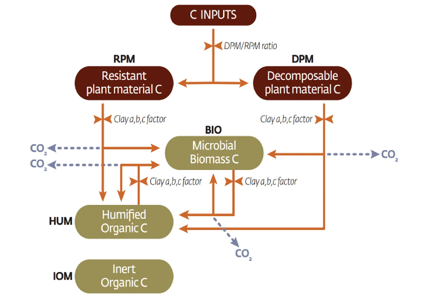
Carbon pools and flows in the RothC model
Figure 1. Carbon pools and flows in the RothC model. Incoming plant carbon is divided between DPM and RPM. Decomposition transfers carbon into BIO and HUM and releases CO2; IOM is represented as an inactive pool. Image source: FAO, Open Knowledge Repository (GSOCseq)link opens in new page.
Model Data Inputs at a Glance
- Climate Data (clima.csv): Monthly air temperature (°C), rainfall (mm), and open pan evaporation (mm).
- Soil Properties (soil_properties.csv): Clay content (%), soil depth (cm), and baseline SOC stock (t C/ha).
- Land Management (inputs_litter_forward_yearly.csv): Monthly plant residue carbon inputs, farmyard manure additions, and soil cover status (bare vs. vegetated).
SOC Modeling Using RothC - Practical Guide
This toolbox can be run either with the R programming language or using a posit.cloud project.
You can download the necessary project files from herelink opens in new page
Go to the website https://posit.cloud/link opens in new page and follow these instruction steps for posit.cloud herelink opens in new page.
Understanding the RothC Modeling Process
Soil Organic Carbon (SOC) modeling with RothC involves two main phases: an Initialization Phase (spin-ups) to estimate unknown initial soil conditions, followed by a Forward Modeling Phase to project future soil carbon dynamics.
Phase 1: Spin-up and Initialization Scheme
In most real-world scenarios, we only measure total SOC from a soil sample (e.g., 15.2 t C/ha). However, RothC does not treat SOC as a single uniform mass. Instead, it divides soil organic matter into five distinct pools:
- DPM: Decomposability Plant Material (fast-decaying, e.g., fresh leaves/succulent residues)
- RPM: Resistant Plant Material (slow-decaying, e.g., woody or fibrous residues)
- BIO: Microbial Biomass (living soil microbes)
- HUM: Humified Organic Matter (stable, long-term soil carbon)
- IOM: Inert Organic Matter (highly resistant carbon, virtually inactive over decades)
Because field samples only give us total SOC and not the exact breakdown among these five pools, we use a two-step spin-up procedure to mathematically determine the starting sizes of each pool.
Super Long Spin-up (Cinput=1):
We run the model for thousands of simulated years (typically 10,000 years) using a dummy annual carbon input rate of exactly 1 t C/ha/year under long-term historical baseline climate conditions.
PRACTICAL STEP FOR BEGINNERS
- Open the input table inputs_litter_forward_yearly.csv.
- Set Month 9 (September) Plant Carbon input to 1.0. Set all other months (1–8 and 10–12) to 0.0.
- Ensure all Exogenous Organic Matter (EOM / manure) columns are set to 0.0 for all months.
- Run the R script EcoSocMan_v00.Rmd for 10,000 years (120,000 monthly steps).
Why do this? Running the model for 10,000 years with a total annual input of 1 t C/ha ensures that all active carbon pools reach mathematical steady state (equilibrium), where annual carbon decomposition exactly equals annual carbon input.
2. Calculating Total Simulated SOC & Deriving Ceq:
Under steady-state conditions, RothC behaves linearly with respect to carbon inputs. This means if you double the input, all active pools double in size.
To find the exact annual equilibrium carbon input (Ceq) required for your soil:
- Obtain SOCsimulated,unit: Sum the simulated pool sizes at the end of month 120,000 (year 10,000) from the model output (DPM + RPM + BIO + HUM + IOM).
- Obtain SOCtarget: Read the measured target SOC stock (in t C/ha) directly from the SOC column in soil_properties.csv.
- Calculate Ceq ratio: Divide the target measured SOC by the simulated unit SOC:
Ceq=SOCtarget/SOCsimulated,unit
Worked Calculation Example:
- Target measured SOC stock from soil_properties.csv (SOCtarget) = 15.2 t C/ha
- Simulated SOC at Year 10,000 with unit input 1 (SOCsimulated,unit) = 6.47 t C/ha
- Calculate Ceq: Ceq=15,2/6,47=2,35 t C/ha/year
Interpretation: The soil requires an average annual carbon addition of 2.35 t C/ha/year to sustain a total SOC stock of 15.2 t C/ha under these climate conditions.
3. Shorter Spin-up / Pool Stabilization (Replacing Unit Inputs with Ceq):
Next, a second spin-up simulation is run across a shorter historical timeline (e.g., from 1850 or 1901 up to the start of your observation period). In this step, we replace the dummy input with the calculated Ceq value.
Why do this? While the long spin-up establishes baseline equilibrium, this shorter historical run with accounts for modern weather variability and historic management trends leading up to the present day. This stabilizes and calibrates the exact starting sizes for all five individual carbon pools (DPM, RPM, BIO, HUM, IOM) immediately prior to your project start date.
Phase 2: Forward Modeling and Management Scenarios
Once the initialization phase establishes accurate starting pool sizes in forward_initial_poolsize.csv, we execute the forward projection.
Simulation Period:
The model is run forward in monthly time-steps across your desired forecast window (e.g., up to the year 2050 or 2100) using actual monthly climate data from clima.csv.
Evaluating Management Practices:
Forward modeling is typically run under multiple management scenarios to compare outcomes:
- Business-As-Usual (BAU): Continuation of standard baseline agricultural practices.
- Sustainable Soil Management (SSM): Adoption of practice changes designed to increase SOC, such as introducing cover crops, applying organic amendments (manure/compost), reducing tillage frequency, retaining crop residues, or introducing agroforestry.
Comparing these scenario outputs reveals the net soil carbon sequestration potential over time.
Explore the workshop exercises
Three exercises connect model inputs with carbon trajectories. Compare the scenarios, interpret the results and explore the questions at the end of each page.
Soil carbon under drought: the O3HP rain exclusion experiment
How can reduced rainfall change the amount of carbon stored in forest soil? This exercise uses the RothC model to explore soil organic carbon (SOC) dynamics under natural drought and experimentally amplified drought at O3HP.
1. The experiment
O3HP (Oak Observatory at the Observatoire de Haute-Provence) is an experimental forest site in southern France, dominated by downy oak (Quercus pubescens). Its rain exclusion system creates drier conditions within an established Mediterranean forest, allowing researchers to examine ecosystem responses to prolonged water limitation.
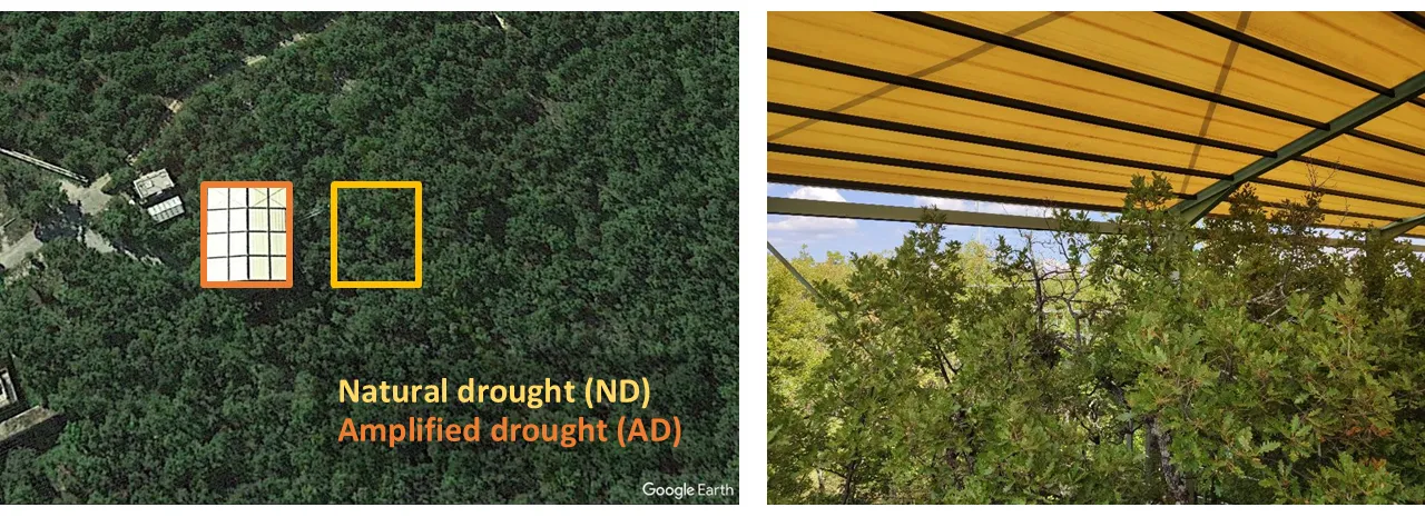
Two treatments are compared: natural drought (ND), exposed to ambient rainfall and the normal Mediterranean dry season, and amplified drought (AD), where a roof above the canopy intercepts selected rainfall events. Rain exclusion began in April 2012 and reduces annual precipitation by approximately 30%, extending the drought period [1, 2].
Figure 1. The O3HP experimental site. The aerial view locates the ND plot (yellow outline) and AD plot (orange outline); the photograph shows the roof used to exclude rainfall.
2. The modeling exercise
The objective is to compare how SOC develops under the two treatments over approximately 100 simulated years. RothC tracks carbon in five pools—decomposable and resistant plant material, microbial biomass, humified organic matter, and inert organic matter. Carbon enters through organic inputs and leaves through decomposition; temperature, moisture and soil cover regulate decomposition in the model.
| Component | Role in the exercise |
|---|---|
| Starting conditions | Initialize the model pools using the spin-up procedure described in the practical guide. The displayed simulations begin at a similar total SOC stock, approximately 23 t C ha−1. |
| Litter inputs | Use the ND and AD litter records to define treatment-specific carbon inputs. If the records represent dry litter mass, convert them to carbon mass using an appropriate carbon fraction. |
| Climate and soil | Supply monthly temperature, rainfall and evaporation, together with clay content, soil depth and soil cover. Treatment-specific rainfall can represent rain exclusion. |
| Forward simulation | Run monthly simulations and compare total SOC and the difference between treatments. State how climate and litter inputs are extended beyond the observation period. |
3. Results and interpretation
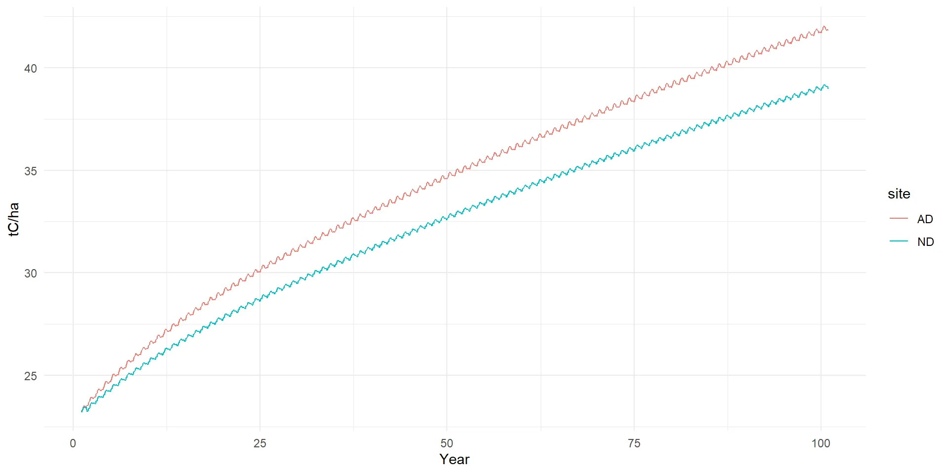
Figure 3. Simulated SOC trajectories under AD (coral) and ND (turquoise). The horizontal axis represents simulation years. Values below are approximate readings from the supplied figure.
SOC increases in both simulations, reaching approximately 42 t C ha−1 under AD and 39 t C ha−1 under ND after about 100 years. The treatments progressively diverge, with AD ending roughly 3 t C ha−1 higher. Small seasonal fluctuations accompany the long-term accumulation, and neither curve appears to have reached equilibrium by the end of the simulation.
The higher modeled SOC under AD is consistent with its generally greater litter inputs. Reduced moisture could also slow decomposition if the rainfall treatment is represented in the model forcing. The plotted trajectories show the combined outcome of the settings used; their separate contributions can be explored by changing rainfall while holding inputs constant, and then changing inputs while holding climate constant.
Main lesson: Drought can affect both the supply of organic material and its decomposition. In this exercise, the modeled balance produces greater SOC accumulation under AD. The century-long trajectories are scenario projections under the selected assumptions, rather than a century of field measurements.
Explore further: Does AD still accumulate more SOC when both treatments receive the same litter carbon inputs?
Experiment background
[1] Saunier et al. (2017). Chronic Drought Decreases Anabolic and Catabolic BVOC Emissions of Quercus pubescens in a Mediterranean Forest. Frontiers in Plant Science, 8, 71. doi:10.3389/fpls.2017.00071link opens in new page
[2] Amplified Drought and Seasonal Cycle Modulate Quercus pubescens Leaf Metabolomelink opens in new page (2022).
Figures supplied for this exercise. Experiment references support the site description; simulation results are interpreted from the supplied SOC figure.
Soil carbon after a bark beetle outbreak:the Plešné and Čertovo forest catchments
What happens to soil carbon when a forest experiences widespread tree mortality? This exercise uses RothC to explore how contrasting litter inputs influence simulated soil organic carbon (SOC) in two Norway spruce forest catchments in the Czech Republic.
1. The study
The exercise draws on Kopáček et al. (2015), who investigated litterfall chemistry and fluxes, together with cellulose decomposition, in mature, unmanaged Norway spruce (Picea abies) forests in the catchments of Plešné Lake (PL) and Čertovo Lake (CT) during 2003–2013. These are two forest catchments, each with its own environmental conditions and history.
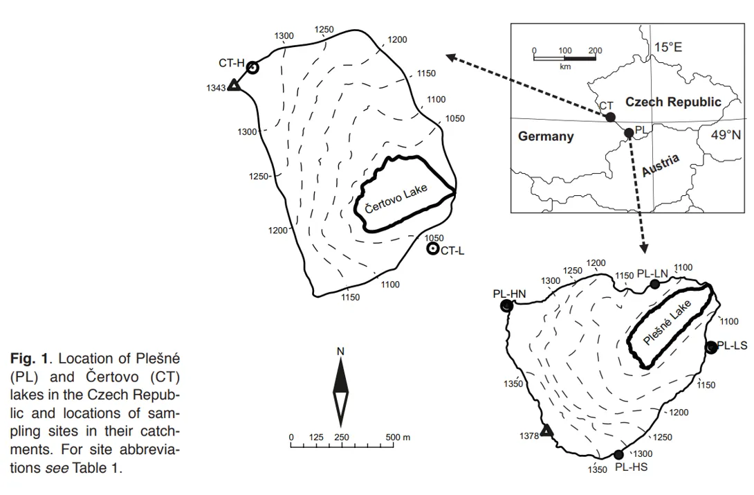
Figure 1. Location of the two lake catchments and their sampling sites. The litter input series used in this exercise are labelled CT-L and PL-LS. Map reproduced from the supplied study material.
The Plešné forest was infested by the bark beetle Ips typographus in 2004, and 88–99% of trees had died by 2011. The study reported a rise in total litterfall from approximately 5.4 to 42 t ha−1 yr−1 after infestation. Litterfall remained relatively high at the end of the study, while litter composition also changed and cellulose decomposition increased [1].
[1] Kopáček J., Cudlín P., Fluksová H., Kaňa J., Picek T., Šantrůčková H., Svoboda M. & Vaněk D. (2015). Dynamics and composition of litterfall in an unmanaged Norway spruce (Picea abies) forest after bark-beetle outbreak. Boreal Environment Research 20: 305–323. Journal abstract and full-text accesslink opens in new page.
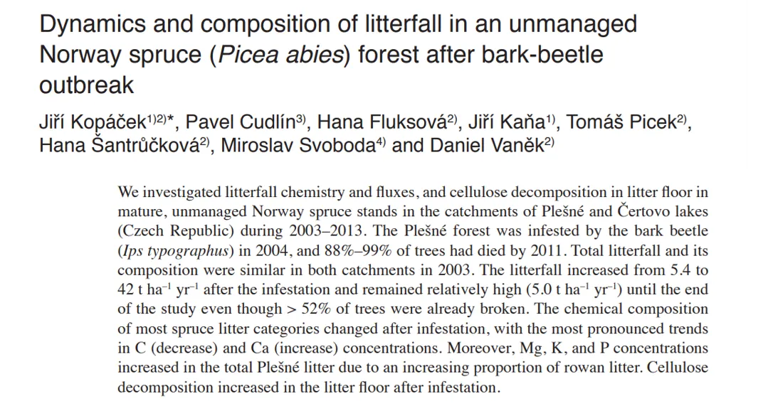
Figure 2. Source paper for the case study. The field study documents the disturbance and litterfall response; the RothC output below belongs to the modeling exercise.
2. From litterfall to model inputs
Tree mortality can generate a large transfer of organic material from the canopy to the forest floor. The litter series illustrates this pulse: PL-LS inputs increase sharply around 2006–2007, reaching approximately 465 mmol C m−2 day−1, whereas CT-L inputs remain comparatively stable, mostly around 25–60 mmol C m−2 day−1. Later PL-LS inputs decline and sometimes fall below CT-L.
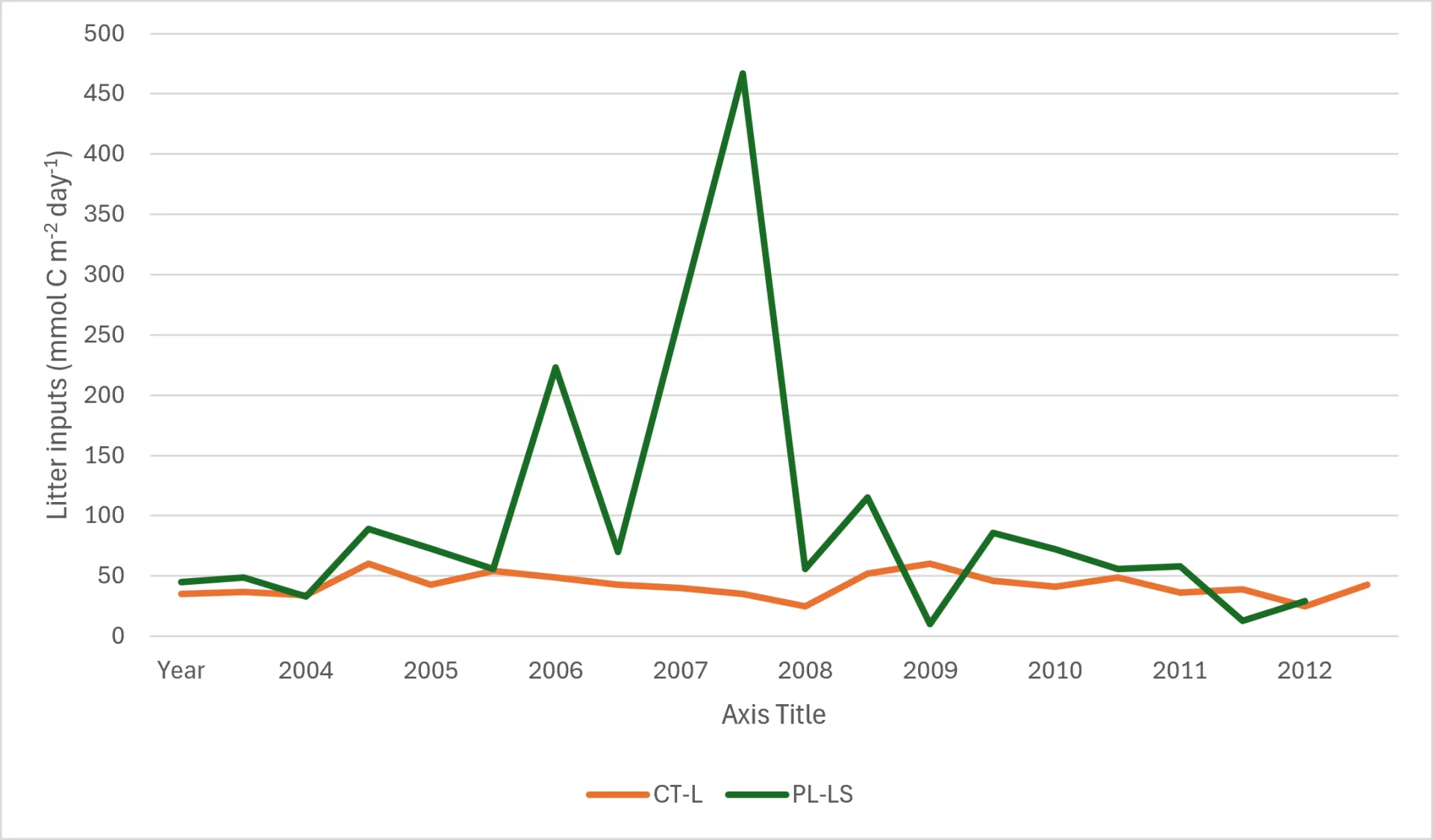
Figure 3. Litter carbon inputs for CT-L (orange) and PL-LS (green). The vertical axis expresses carbon flux in mmol C m−2 day−1; the horizontal labels show the observation period. Values are read approximately from the supplied graph.
These inputs already express carbon rather than total dry litter mass. To prepare them for RothC, convert the daily flux to the carbon amount entering during each monthly timestep. For a mean daily flux F representative of a whole month:
Monthly input (t C ha−1) = F × 0.00012 × days in the month
The factor converts mmol C m−2 to t C ha−1, using 12 g C mol−1. For example, 50 mmol C m−2 day−1 over 30 days supplies 0.18 t C ha−1.
3. The modeling exercise
The objective is to examine how a disturbance-related litter pulse is reflected in soil carbon dynamics. RothC distributes incoming carbon among decomposable and resistant material and tracks its transfer into microbial biomass and humified organic matter, alongside an inert pool. Climate, soil moisture, soil cover and clay content influence the resulting carbon balance.
| Step | Practical task |
|---|---|
| Initialize the soil | Use the spin-up procedure in the practical guide to estimate starting carbon pools for each site. Retain each site's initial SOC when comparing changes. |
| Prepare inputs | Convert litter carbon fluxes to monthly amounts and assign their timing and decomposability. State how any additional inputs, such as roots, are represented. |
| Run the model | Supply monthly climate, soil properties and cover information, then simulate the two site cases. Record which settings differ between them. |
| Compare responses | Examine total SOC, seasonal fluctuations and change from each site's starting stock. Use a run without the litter pulse to explore its contribution. |
4. Results and interpretation
| Series | Initial value | Final value | Approximate change |
|---|---|---|---|
| TC_PL | 143 | 133 | −10 (about −7%) |
| TC_CT | 131 | 111–112 | −19 to −20 (about −15%) |
Both simulations lose carbon, but PL declines less and shows more pronounced fluctuations. This pattern is consistent with larger litter inputs partly compensating for decomposition losses. The graph illustrates that an input pulse need not produce a sustained rise in total SOC: carbon can continue to decline when losses exceed additions.
PL also begins with more carbon, so the final gap includes an initial difference as well as differences that develop during the simulations. Comparing changes from the starting values helps interpret the trajectories; a separate simulation with the same starting pools and climate, but without the disturbance pulse, would isolate the modeled effect of that pulse.
Main lesson: Widespread tree mortality can temporarily increase litter supply and buffer soil carbon losses. Higher litter inputs reflect the transfer of carbon from damaged trees, and do not by themselves demonstrate greater productivity or a gain in total forest carbon.
Explore further: How would the PL trajectory change if the large litter pulses were replaced by its pre-outbreak input rate?
Forest soil carbon under disturbance and climate scenarios
How do disturbance, forest management and changing climate conditions alter soil carbon trajectories? This exercise compares hypothetical scenarios over 100 simulation years, using the Swabian Alb as a geographical setting.
Entirely simulated data. All data in this exercise are simulated for teaching. The curves illustrate the behavior of the selected model scenarios; they are not field observations or validated forecasts for forests in the Swabian Alb.
1. Aim and model framework
The aim is to explore how changes in carbon inputs and decomposition can produce different soil organic carbon (SOC) stocks and soil CO2-C release rates. RothC represents soil carbon in five pools: decomposable plant material, resistant plant material, microbial biomass, humified organic matter and inert organic matter. The balance between carbon additions and decomposition determines whether modeled SOC increases or decreases.
The exercise contrasts a baseline with hypothetical drought, beetle disturbance, deadwood, management and climate cases. The names identify their intended themes; the magnitude, timing and duration of each change depend on the scenario settings. Labels alone do not specify mortality rates, input pulses, replanting rates or climate adjustments.
2. The scenarios
The main characteristics below describe the intended scenario concepts and, where available, the responses visible in the figure. Exact changes in inputs, climate, mortality and recovery must be taken from the simulation settings.
| Code | Scenario | Main characteristics | Shown |
|---|---|---|---|
| A | Baseline growth | Reference case with continuing forest growth and organic carbon inputs, without an imposed beetle outbreak or clear-cut. Provides the benchmark for assessing disturbance and climate responses. | Yes |
| B | Unmanaged beetle | Beetle-related tree mortality without subsequent harvesting or replanting. The conceptual response combines an initial supply of dead plant material with reduced inputs from living trees and subsequent natural recovery. | No |
| C | Drought only | Water limitation without a beetle outbreak. Drought can affect both plant carbon inputs and moisture-dependent decomposition; their balance determines the SOC response. The displayed trajectory largely returns to the baseline. | Yes |
| D | Drought + beetle | Combined water limitation and beetle disturbance. The displayed case has a large early carbon pulse, a strong CO₂-C release peak, prolonged SOC depletion and later partial recovery. | Yes |
| E | Gradual deadwood decay | A gradual supply of carbon from decaying deadwood rather than transferring all deadwood carbon into the soil at once. Emphasizes the timing of carbon transfer and its influence on soil inputs and decomposition. | No |
| F | Clear-cut + replanting | Tree removal followed by establishment of a new stand. Conceptually combines reduced living-tree inputs after cutting with increasing inputs during regrowth; the amount of retained harvest residue depends on the scenario settings. | Yes |
| G | Repeated beetle outbreaks | Successive disturbance events interrupt recovery. In the displayed simulation, responses occur around years 20 and 55, allowing comparison of repeated disturbance with a single event. | Yes |
| H | RCP2.6 | Climate case labelled RCP2.6, representing the lower-forcing member of the three RCP cases. Intended for comparison of SOC responses under alternative climate assumptions. | No |
| I | RCP4.5 | Climate case labelled RCP4.5, representing intermediate forcing among these three cases. The displayed simulation ends below the baseline SOC stock but above RCP8.5. | Yes |
| J | RCP8.5 | Climate case labelled RCP8.5, representing the highest forcing among these three cases. The displayed simulation ends with the lowest SOC stock of the two RCP cases shown. | Yes |
The figure displays seven of the ten defined scenarios. The RCP names describe the intended climate cases, rather than specifying the actual climate data used here. Temperature, rainfall and evaporation changes, and any associated changes in plant inputs, must be checked in the simulation settings. These entirely simulated trajectories are not validated RCP projections for the site.
3. Read the two outputs together
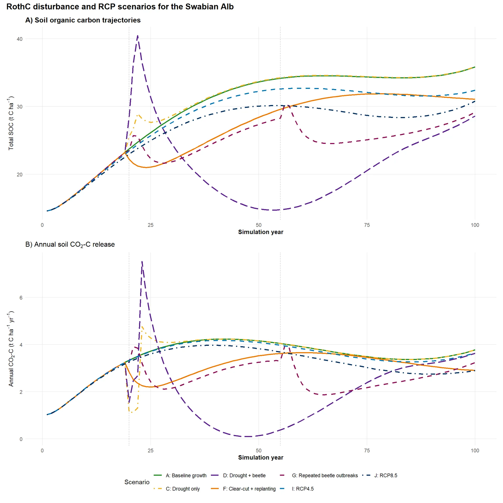
Figure 1. Entirely simulated RothC disturbance and climate scenarios for a teaching exercise set in the Swabian Alb. Upper panel: total SOC (t C ha−1). Lower panel: annual soil CO2-C release (t C ha−1 yr−1). Dotted vertical lines mark approximately simulation years 20 and 55. Panel labels A and B refer to the two outputs; scenario codes A–J refer to the legend and table above.
SOC is a stock: it describes carbon present in the modeled soil at a given time. Annual CO2-C release is a flux: it describes carbon released as CO2 during a year. Its units express the mass of carbon in CO2, rather than the mass of the whole CO2 molecule.
4. Results and interpretation
Baseline growth (A) increases SOC from roughly 15 to 36 t C ha−1. The drought-only case (C) departs temporarily from the baseline around year 20, then largely converges with it. Under these simulated settings, the isolated drought effect is relatively short-lived.
Drought + beetle (D) produces the strongest transient response. SOC briefly exceeds 40 t C ha−1, then falls to approximately 15 around years 50–55 before recovering to about 29 by year 100. Annual CO2-C release peaks above 7 t C ha−1 yr−1, then declines almost to zero before rising again. This pattern is consistent with a large input pulse followed by depletion and later recovery, although its precise cause must be traced to the input and decomposition settings.
Clear-cut + replanting (F) causes an initial decline to about 21 t C ha−1, followed by recovery to roughly 31 at the end of the simulation. Repeated beetle outbreaks (G) create distinct responses around years 20 and 55, interrupting recovery and leaving SOC near 29 at year 100.
The RCP4.5 (I) and RCP8.5 (J) cases finish at approximately 32 and 31 t C ha−1, respectively, below the baseline. In this exercise, J also has lower late-period annual CO2-C release than A. This shows why the two outputs must be interpreted together: lower release can occur alongside a smaller soil carbon stock.
Main lesson: A temporary carbon pulse, a high final SOC stock and low annual CO2-C release describe different aspects of a trajectory. Assess the size of the disturbance response, recovery time and long-term stock together. Soil outputs alone do not establish the carbon balance of living trees, deadwood, harvested products and the whole forest ecosystem.
5. Explore the scenarios
- Compare each scenario with A at the same simulation year. Which has the greatest temporary departure, and which has the largest final SOC deficit?
- For D, compare SOC and annual CO2-C release before the disturbance, at the emission peak and near the SOC minimum. How does the interpretation change across these stages?
- Compare F and G: which recovers more strongly by year 100, and how would the answer depend on the chosen assessment year?
- Inspect the scenario inputs and rerun one case with only a single factor changed. Which features of the curves can you attribute to that change?